ラウエ関数(干渉関数)

Laue function (interference function)

反射波の振幅が格子面(結晶面)の数とともにどのように変化(増大)していくかを、反射の励起誤差の関数(ロッキングカーブという)として表したもの。反射の主極大 (中央のピーク)は格子面の数の二乗に比例する。副極大は格子面の数と共に急速に減少する。
通常、反射に関与する格子面の数は十分多いので副極大は極端に小さくなり実際に観察されることはない。さらに、電子回折では、多重散乱による動力学回折効果のために、ロッキングカーブはラウエ関数とは異なる関数になる。主極大は有限に留まり、副極大は大きな強度を持って観察される。実際のロッキングカーブは動力学回折理論によって説明される。

ラウエ関数 G の導出

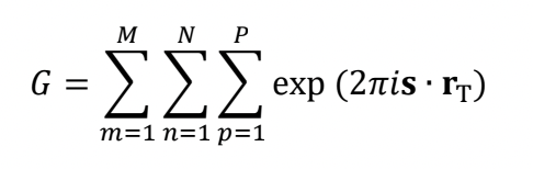
ブラッグ反射g からの“はずれ”に対して反射の振幅がどのように減衰するか(ロッキングカーブ)を見るために、ブラッグ条件からの外れの量(励起誤差)をsとして、k − k₀ = g + s とおいて、各格子面からの位相を結晶全体にわたって加算する。

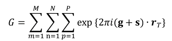
ここで、m,n,p は、x,y,z の三方向の格子の指数を表し、和の上限を M,N,P とする。r_T は T 番目の格子の座標を表すベクトルである。格子点からのブラッグ反射 g は全て位相が揃っているので、g ∙ r_T= 整数であるから、上の式は

となる。この式は g を含んでいないので、全ての反射に同じ効果を与える。三方向 (i =1.2.3) に対して別々に和をとったあと、位相因子を除くと次式のようになる。

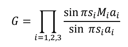
ここで、a_i は単位胞の格子定数、M_i は格子の数の最大値である。G の二乗が強度を表すので、主極大(s_i = 0)は M_i²になる。すなわち、結晶の大きさ (厚さ) の二乗に比例する。図 1 にラウエ関数の例を示す。

図 1:ラウエ関数の M=5 および M=60 の例。主極大が M の二乗に比例しているのが分かる。M の増加と共に、主極大はシャープになり、副極大は小さくなる。(田中通義、寺内正己、津田健治:「やさしい電子回折と初等結晶学」(共立出版)、2014 より転載)

実際に観察されるロッキングカーブ

実際に観察される回折強度の角度変化(ロッキングカーブ)はラウエ関数とは異なる。その理由は結晶に入射した電子線は結晶中で多数回散乱を繰り返すからである。実際のロッキングカーブは多重散乱を考慮した理論である動力学回折理論によって説明される。
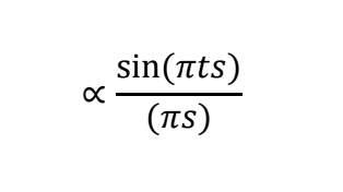
上で示したラウエ関数を 1 次元で表して、s を小さいとして分母の sin πs を πs と近似して、M_a = t と置くと

となる。
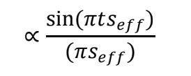
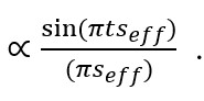
動力学回折理論によれば、ラウエ関数は次の式に置き換えられる(詳しくは文献 1 を参照)。

ここで、

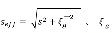
は消衰距離といわれるもので以下のように与えられる。

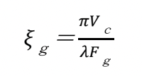
ここで、V_c は結晶の単位胞の体積である。ξ_g は結晶構造因子 F_g に反比例する量である。図 2に、ラウエ関数(運動学的ロッキングカーブ)と動力学的ロッキングカーブを示す。ラウエ関数では、主極大は結晶の厚さの二乗に比例して大きくなるが、その半値幅は厚さに反比例して小さくなる。他方、動力学回折理論によれば、s_eff の中にξ_g があるために、厚さが増してもs=0 で強度が発散することなく有限の値にとどまり、副極大は図に示すような包絡線に沿って減少する。さらに、図に示すように、s=0 で強度が最大になるとは限らない。

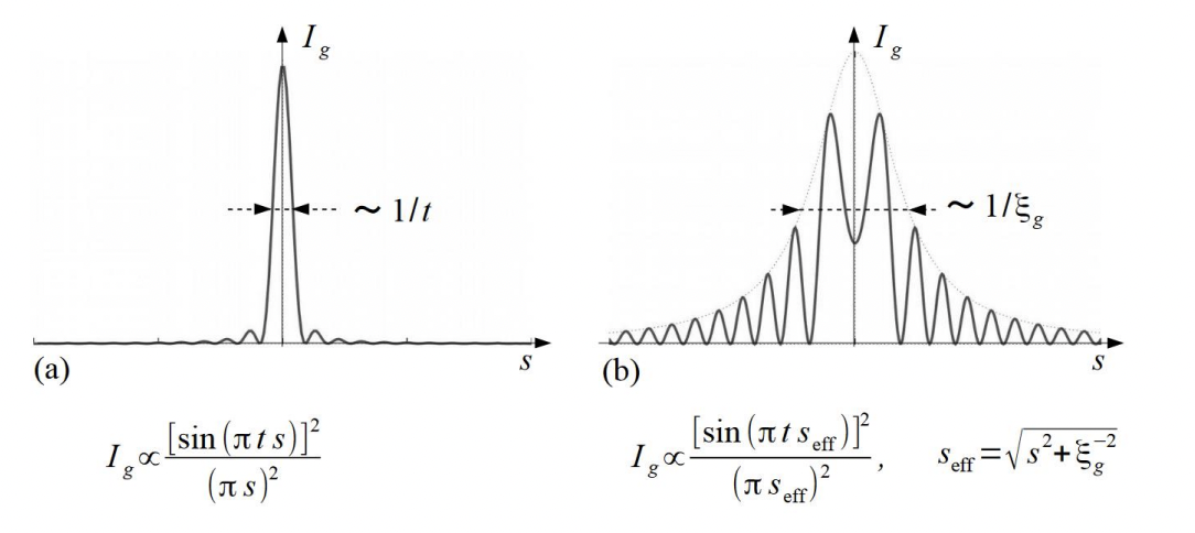
図 2: (a) ラウエ関数(運動学的ロッキングカーブ) と (b)動力学的ロッキングカーブ
(田中通義、寺内正己、津田健治:「やさしい電子回折と初等結晶学」(共立出版)、2014 より転載)
図 3 に実際のロッキングカーブを示す。図 2 に示したロッキングカーブと似た強度の角度変化が見られる。

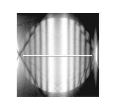
図 3:Si の 220 反射のロッキングカーブ。図 2(b)に対応した強度変化が観察されている。(田中通義、寺内正己、津田健治:「やさしい電子回折と初等結晶学」(共立出版)、2014 より転載)

文献 1: M. J. Whelan, Dynamical Theory of Electron Diffraction, in "Diffraction and Imaging Techniques in Material Science", eds. S. Amelinckx, R. Gevers and J. van Landuyt (North-Holland Publishing Company,1978, ISBN: 978-0-444-85128-4)

The Laue function (interference function) expresses how the amplitude of a reflected (diffracted) wave increases with increasing the number of lattice planes (crystalline planes), as a function of the excitation error of the reflection (called “rocking curve”). The magnitude of the principal maximum of the reflection (central peak) is proportional to the square of the number of lattice planes. The subsidiary maxima rapidly decrease with increasing the number of lattice planes. Normally, as the number of lattice planes contributing to the reflection is sufficiently large, the subsidiary maxima become extremely small and are not actually observed. Furthermore in electron diffraction, owing to the dynamical diffraction effect due to multiple scattering, the real rocking curve is different from the Laue function. The principal maximum stays finite and subsidiary maxima are observed with great intensities. The rocking curve really observed is interpreted by the dynamical diffraction theory.

Derivation of the Laue function G

In order to examine how the amplitude of a Bragg reflection g is decreased against the deviation from the Bragg reflection (rocking curve), the deviation parameter s from the Bragg angle (excitation error) is introduced and k − k₀ = g + s. The phases from the lattice planes are added over the whole crystal.

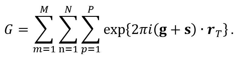
Here, m,n,p express the lattice indices in the three directions of x,y,z,and the sums are taken up to M,N,P. r_T is the distance of the T-th lattice point. Since at a Bragg condition, the reflections from all the lattice points are in phase, g・r_T=an integer. Then, the above equation is written as follows.

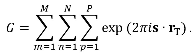
This equation does not include g and thus, G is common to all of the reflections. The three summations (i =1.2.3) can be performed separately. By removing the phase factors, finally the next equation is obtained.

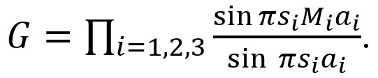
Here, a_i is the lattice parameter of the unit cell, and M_i is the maximum number of the lattice. The square of G gives the intensity from the crystal lattices, and the principal maximum (s_i = 0) is M_i². That is, the principal maximum is proportional to the square of the size (thickness) of the crystal. Fig. 1 shows two examples of the Laue function.

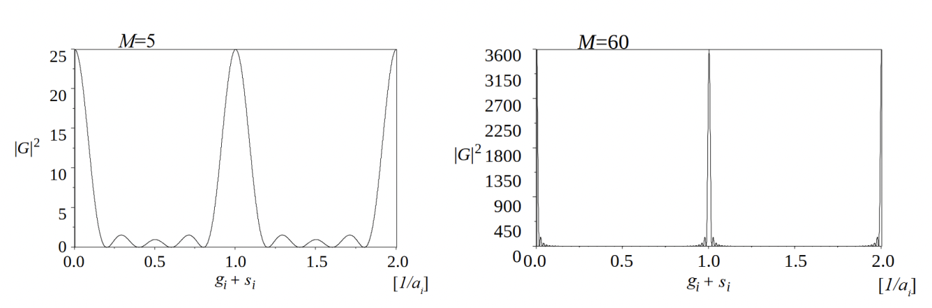
Fig. 1. Example of the Laue functions for M = 5 and M = 60. The principal maximum is seen to be proportional to the square of M. With the increase of M, the principal maximum becomes sharper and the subsidiary maxima become smaller as is seen in the case of M = 60. (reprinted from M. Tanaka, M. Terauchi, K. Tsuda,“Introduction to Electron Diffraction and Elementary Crystallography (in Japanese)”, Kyoritsu Printing Co.,Ltd., 2014)

Rocking curve actually observed

The angular dependence of the diffraction intensity (rocking curve) actually observed is different from the Laue function. This is because the incident electron beam suffers multiple scattering in the crystal. The rocking curve is explained by the dynamical diffraction theory taking multiple scattering effect into account.
Let us write the Laue function in one dimensional manner, and assume s to be small and approximate sin πs as πs. Then, the following equation is obtained.

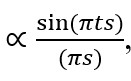
where Ma = t.
According to the dynamical diffraction theory, the Laue function is replaced by the following equation (for details, refer to Ref. 1),

Here,

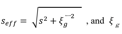
is called “extinction distance” and given by

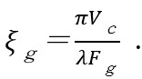
Here, V_c is the volume of the unit cell of the crystal. It is noted that ξ_g is inversely proportional to the crystal structure factor F_g.
Fig. 2 shows examples of the Laue function (kinematical rocking curve) and the dynamical rocking curve. In the Laue function, the principal maximum increases proportional to the square of the thickness of a crystal, and the width of the principal maximum decreases inversely proportional to the thickness.
On the other hand, the rocking curve obtained by the dynamical diffraction theory is given by a function of s_eff. As a result, even if the thickness increases, the intensity at s=0 does not diverge with the crystal thickness but remains at a finite value, and the subsidiary maxima slowly decrease along the envelope shown in Fig. 2. Furthermore, the intensity at s=0 does not necessarily take the maximum value (shown in Fig.2(b)).

Fig. 2. (a) Laue function (kinematical rocking curve) and (b) dynamical rocking curve. See the explanations in the text.
(reprinted from M. Tanaka, M. Terauchi, K. Tsuda, “Introduction to Electron Diffraction and Elementary Crystallography (in Japanese)”, Kyoritsu Printing Co., Ltd., 2014)
Fig. 3 shows an experimentally obtained rocking curve. It should be noted that the rocking curve shows a good agreement with the dynamical rocking curve shown in Fig. 2(b).

Fig. 3. Rocking curve of the 220 reflection of Si. Angular intensity change is confirmed similar to that in Fig.2(b). (reprinted from M. Tanaka, M. Terauchi, K. Tsuda, “Introduction to Electron Diffraction and Elementary Crystallography (in Japanese)”, Kyoritsu Printing Co., Ltd., 2014)

Ref. 1: M. J. Whelan, Dynamical Theory of Electron Diffraction, in “Diffraction and Imaging Techniques in Material Science”, eds. S. Amelinckx, R. Gevers and J. van Landuyt (North-Holland Publishing Company,1978, ISBN: 978-0-444-85128-4)