元素マッピング(EDS)
元素マッピング(EDS)
Elemental mapping, EDS
[目次:分析]
特性X線を用いた元素分析の方法のひとつ。指定した領域の指定した元素の特性X線の強度分布または元素の濃度分布を二次元的に表示して、試料の元素の分布を可視化する方法。
エネルギー分散型X線分光法 (EDS) による元素マッピングでは、分析対象の領域を電子線で二次元的に走査し、発生する特性X線スペクトルをその画素ごとに取得する。それらのスペクトルから分析対象の元素のX線強度または元素濃度を算出して各画素に表示することで、元素マップを得る (図1)。
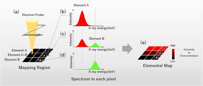
図1 元素マッピングの方法
- (a) 元素Aと元素Bが存在する領域を電子線で二次元的に走査し、画素ごとにX線スペクトルを得る。
- (b) 図 (a) 中の画素 (i) から得られたスペクトル。元素Aの特性X線のエネルギー位置に強いX線ピークが形成されている。
- (c) 図 (a) 中の画素 (ii) から得られたスペクトル。元素A、Bそれぞれの特性X線エネルギー位置にピークが形成されている。
- (d) 図 (a) 中の画素 (iii) から得られたスペクトル。元素Bの特性X線エネルギー位置にピークが形成されている。
- (e) 図 (a) 中の各画素のスペクトルから、元素Aの特性X線の積分強度を抽出、または元素濃度を算出し各画素に表示すると、元素Aの元素マップが得られる。
EDSの元素マップには3種類あり、そのうちの2つは特性X線の強度マップ、1つは元素の濃度マップである。それぞれのマップの特性を、以下の表1に示す。
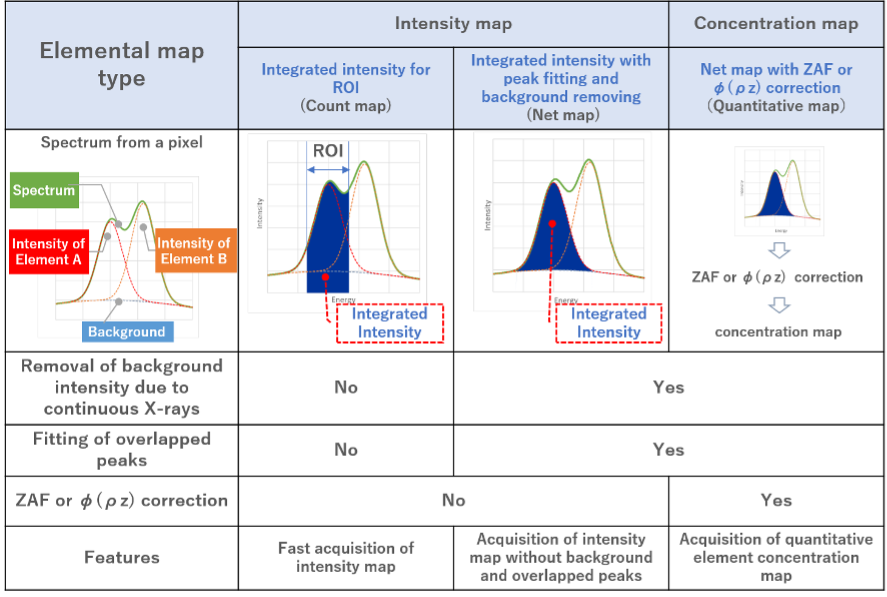
表1 EDSの元素マップの比較表
(I) 特性X線の強度マップ
マッピング領域の各画素のスペクトルから、分析対象の元素の特性X線強度を抽出して表示したもの。強度マップからは、その元素がマッピング領域のどこに多く存在しているかを定性的に知ることができる。これは、同じ条件で電子線が照射された場合に検出される特性X線の強度は、その元素の存在量におおむね比例するためである。
特性X線の強度マップには以下の2種類ある。
(i) ROIの積分強度の分布 (カウントマップ) を表示する方法
元素ごとにエネルギーの広がりの領域 (ROI: Region Of Interest) を設定し、画素ごとにROIのX線強度の積分値を表示する方法である。JEOL製品では「カウントマップ」と表記している。
この方法は、ROI中のX線の強度を積算するという単純な処理なので、簡便に、しかも高速に表示できるのが最大の利点である。
ただし、EDSのエネルギー分解能が約130eV (Mn-Kα 5.9keVに対して) であるため、着目する元素に対するROIに他の元素のROIが重なることがあり、正しくない元素分布を表示することがある。また、連続X線によって形成されるバックグラウンド強度が画素によって大きく異なる場合には、バックグラウンド強度の大きな違いも一緒に示してしまうために、特性X線の強度の違いを正しく示さないマップとなる可能性がある。
(ii) バックグラウンド除去とピーク分離処理をした積分強度の分布 (ネットマップ) を表示する方法
(i) の方法での欠点を除き、元素分布の精度を上げる方法。JEOL製品では「ネットマップ」と表記している。
この方法では、あらかじめ質量濃度が既知の標準試料のスペクトルを取得し、連続X線によるバックグラウンドを除去して、標準スペクトルとして使用する。次に、未知試料を測定し、得られたスペクトルからバックグラウンドを除去する。その後、図2に示すように、二つの元素の標準スペクトルにそれぞれ係数をかけて二つのスペクトルを合成し、未知試料のスペクトルを最も良く再現するように係数の値を決める。こうして、未知試料の重畳しているピークは、二つの元素の特性X線ピークに分離される。元素ごとに算出した係数 (すなわち標準スペクトルに対する未知試料のスペクトルの強度の比) に標準スペクトルの積分強度値を掛けると、未知試料のスペクトルから特性X線の積分強度を算出できる。これらの処理を画素ごとに実行することで、対象元素の特性X線の強度分布が得られる。
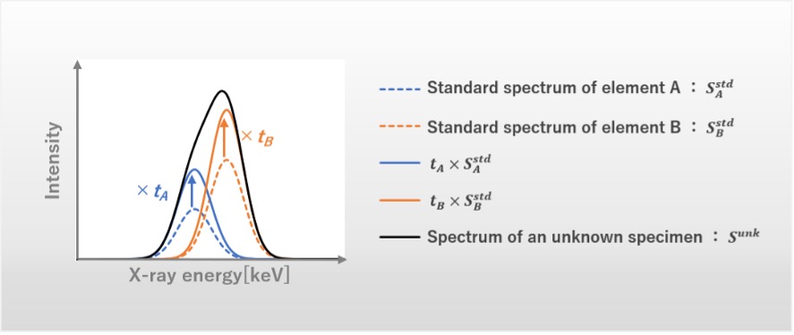
図2 ピーク分離の概念図
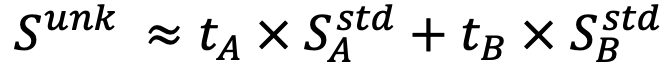
①Sunkをもっともよく再現する係数tAとtBを次の式から求める
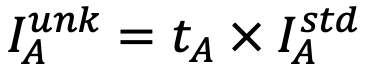
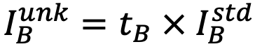
②未知試料に含まれる元素AとBの積分強度 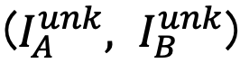 を次の式から求める
ただし、 と
と は、元素AまたはBの標準スペクトルから求めた積分強度である
(II)元素濃度マップ (定量マップ)
マッピング領域の各画素について元素濃度を算出して表示したもの。一般的に、「定量マップ」と表記される。
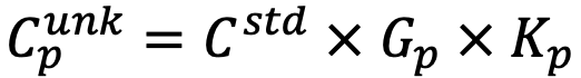
元素濃度マップ (定量マップ) は以下のような方法で求める。まず、各画素 (p) におけるスペクトルのX線強度を、標準スペクトルと同等の測定条件で取得した強度となるように規格化する。次に、ネットマップと同様の方法で係数 (tp) を求める。規格化した状態で求めた係数は、標準試料と未知試料のX線強度比で、Kレシオ(Kp)と呼ばれる。さらに、標準試料と未知試料での共存する元素の違いによるX線強度の違いを表す補正因子 (Gp) をZAF補正やφ (ρz) 法を使って求める。標準試料の濃度をCstdとすると、各画素 (p) における元素濃度  は、次式から求まる。
(詳細は、関連用語「定量補正」「ZAF補正」「ファイローゼット法φ(ρz)法)」を参照)
実際の分析例 : SnPbBi合金の強度マップおよび濃度マップ
ROIの積分強度の分布 (カウントマップ) を表示する方法での欠点を、バックグラウンド除去とピーク分離処理 (ネットマップ) によって改善した事例を紹介する。
図3 (a) はSnPbBi合金の反射電子組成像である。緑、赤、青で示した矩形領域でX線スペクトルを測定した。緑の領域からはSnのスペクトル、赤の領域からはPbのスペクトル、青の領域からはBiのスペクトルが観察された。Snのピークのエネルギー領域はPbやBiのエネルギー領域と重複していないが、PbとBiのピークのエネルギー領域は重複している。そのため、ROIの強度を積分する方法で元素マップを作成すると、PbとBiのROIが重複して図4の左列のようにPbとBiの存在場所が区別できないマップとなる。
他方、ピーク分離処理によって積分強度を表示する方法を用いると、図4の中央列のようにPbとBiの存在を明瞭に分離して示せる。なお、右列の元素マップは濃度マップである。この場合には、濃度マップはネットマップとほとんど変わらないが、それぞれの領域の濃度を、右のカラースケールを使って、定量的に示すことができる。
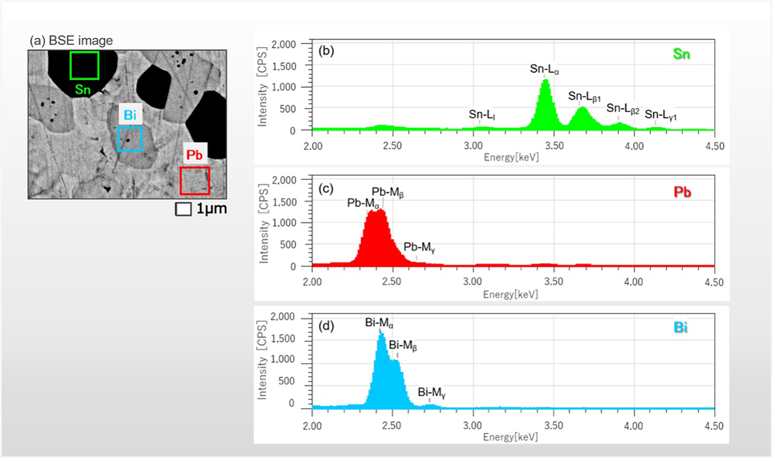
図3 SnPbBi合金の反射電子像とそのX線スペクトル
- (a) SnPbBi合金の反射電子組成像
- (b), (c), (d) 図 (a) 中の緑、赤、青の領域から測定したX線スペクトル。「Sn-Lα」などのラベルはSiegbahnにより命名された特性X線の名称であり、電子の遷移過程を示している。例えば「Sn-Lα」は、L殻のp軌道にできた空孔にM殻のd軌道の電子が遷移したことにより発生した特性X線を表している。
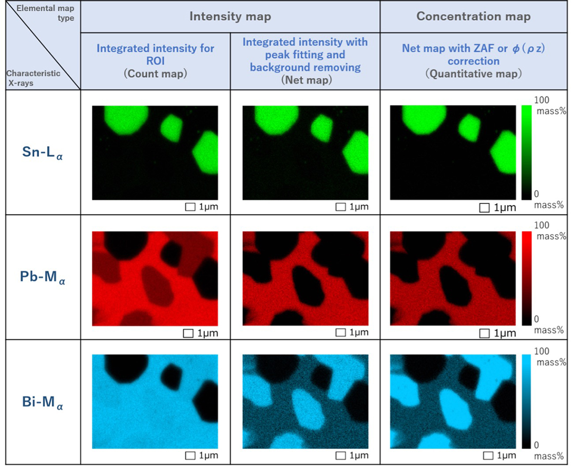
図4 カウントマップ (左列)、ネットマップ (中央列) と定量マップ (右列) の3種類の方法で作成した
Sn-Lα、Pb-Mα、Bi-Mαの元素マップ。
Snの分布については、3種類のマップで差は見られない。
Pbのネットマップ・定量マップは、Pbがある領域 (赤) とPbがない領域 (黒) を正しく示している。しかし、カウントマップでは、Biからの特性X線も取り込んでしまうため、本来Pbのない黒い領域の一部にPbが少し存在している (暗い赤) かのように示されている。
Biのネットマップ・定量マップは、Biが多く存在する領域 (青)、Biが存在する領域 (暗い青) 、Biが存在しない領域 (黒) の3領域を正しく示している。しかし、カウントマップでは、共存しているPbからの特性X線も取り込んでしまうため、青と暗い青との区別がほとんど不明になっている。
ただし、この試料には、定量マップのカラースケールで表現されるような連続的な変化はない。
付録 Feを含有する鉱物試料の強度マップと濃度マップの例
元素濃度とX線強度はおおむね比例関係にあるため、ネットマップと定量マップは、似た分布を示すことが多い。しかし、試料によっては、共存する元素によるX線の吸収などの効果のために、ネットマップと定量マップが異なる分布となることがある。
以下に、Feの含有量が異なる2種類の鉱物からなる試料を調べた例を示す。図5は鉱物試料の反射電子組成像である。左側の黒い部分 (領域A) と右側の明るい部分 (領域B) のそれぞれの領域でX線スペクトルを測定した。領域AはFe、Mn、Oからなり、領域BはFe、Sから構成されていることが分かった。ZAF補正を施した定量分析の結果から、領域AのFeの濃度は領域Bよりも高いことが分かった。
これら二つの領域の強度マップとZAF補正を行った濃度マップを図6に示す。二つの強度マップ (左と中央) では、領域Bの方がFeの特性X線強度が高いことを示している。他方、濃度マップ (右) は、領域Aの方がFeの濃度が高いことを示している。この事例から、ZAF補正の重要さが分かる。
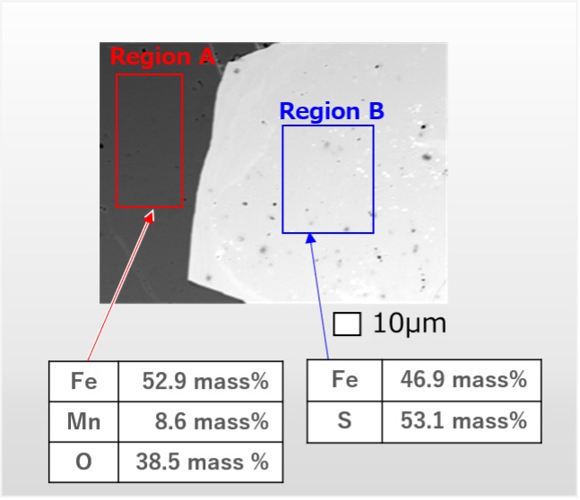
図5 鉱物試料の反射電子組成像
領域A (赤い矩形)、領域B (青い矩形) で測定したX線スペクトルにZAF補正による定量分析を行った結果。領域Aの方が領域BよりFeの濃度が高いことがわかる。
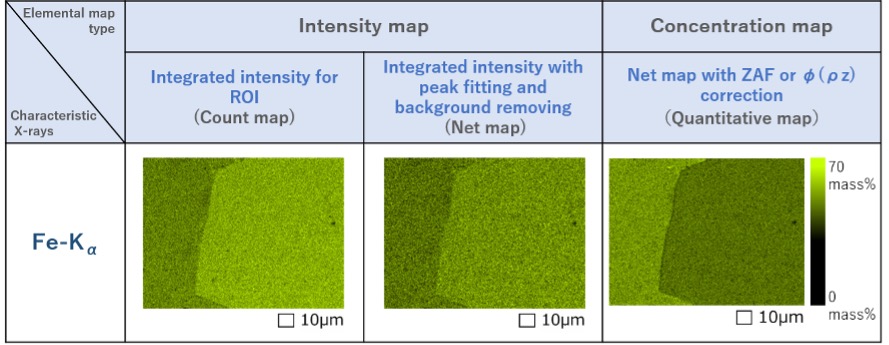
図6 3種類の方法で作成したFeの元素マップ
Fe-KαのX線強度または元素濃度が高い部分を明るい緑色で示し、低い部分を暗い緑色で示している。カウントマップおよびネットマップでは、右側の領域の強度が高くなっているが、定量マップでは右側の領域の濃度が低くなっている。
One of elemental analysis methods using characteristic X-rays generated by an electron-beam. The method visualizes the distribution of the constituent elements in the specimen by two-dimensionally displaying the characteristic X-ray intensities or the concentrations of the elements.
In elemental mapping using energy-dispersive X-ray spectroscopy (EDS), an electron beam is two-dimensionally scanned over a specimen area, and the characteristic X-ray spectra generated by the electron beam are acquired pixel by pixel. From those spectra, the X-ray intensities or the calculated concentrations of the target elements are displayed pixel by pixel, to acquire an elemental map (Fig. 1).
Fig. 1 Procedure of elemental mapping.
- (a) By two-dimensionally scanning an electron beam over an area where element A and element B exist, the X-ray spectra generated from each pixel are acquired.
- (b) Spectrum acquired from pixel (i) in Fig.(a). A strong characteristic X-ray peak of element A is depicted.
- (c) Spectrum acquired from pixel (ii) in Fig.(a). Characteristic X-ray peaks of element A and element B are depicted.
- (d) Spectrum acquired from pixel (iii) in Fig.(a). A characteristic X-ray peak of element B is depicted.
- (e) The integrated intensities of the characteristic X-rays of element A or the element concentrations of element A are plotted pixel by pixel to provide the elemental map of element A.
There are three types of elemental maps using EDS: Two are intensity maps of characteristic X-rays and the third is a concentration map of elements. The features of each map are presented in Table 1.
Table 1 Comparison of the three elemental maps using EDS.
1. Characteristic X-ray intensity map
The map displays the characteristic X-ray intensities of the target elements pixel by pixel. The intensity map qualitatively shows where the elements are more abundant. This is because the intensity of the characteristic X-rays detected under the same condition of electron-beam illumination is roughly proportional to the abundance of the elements.
There are two types of the intensity maps.
1) The first is to display the integrated intensity distribution for ROI (count map).
An energy region for integration (ROI: Region of Interest) is set for each element, and the value of the integrated intensity for ROI is displayed pixel by pixel. At JEOL, the map is called "count map". The advantage of the method is easy and quick to display the map.
However, since the energy resolution of EDS is approximately 130 eV (defined at Mn-Kα 5.9 keV), the ROI of the target element may overlap that of the other element, giving an incorrect elemental distribution. When the background intensities generated by continuous X-rays are largely different from pixel to pixel, the map may not correctly provide the differences of the characteristic X-ray intensities of neighboring pixels due to the large differences in the background.
2) The second is to display the integrated intensity distribution subjected to background removal and peak separation (net map).
This method improves the above method (1) to obtain a better accuracy of the element distribution. At JEOL, the map is called "net map".
The spectrum of a standard specimen with known mass concentrations of constituent elements is measured, and the background due to continuous X-rays is removed. Then, the standard spectrum is prepared. Next, the spectrum of an unknown specimen is measured, and the background due to continuous X-rays is also removed. Then, as shown in Fig. 2, the standard spectra of the two elements are each multiplied by a factor and the two spectra are combined. The values of the two factors are determined so as to best reproduce the spectrum of the unknown specimen. As a result, the overlapping spectra of the unknown specimen are separated into the spectra of the two elements.
By multiplying the factor calculated for each element (i.e. the ratio of the intensity of the spectrum of the unknown specimen to that of the standard spectrum) by the integrated intensity of the element of the standard specimen, the integrated intensity of the element of the unknown specimen is obtained. By performing the procedure for every pixel, the intensity distribution of the characteristic X-rays of the target element is obtained.
Fig. 2 Schematic diagram of peak separation.
1) Factors tA and tB, which reproduce the spectrum of the unknown specimen Sunk, is obtained from the equation
2) The integrated intensities from element A and element B of the unknown specimen are obtained from the equations
where, and are the integrated intensities from element A and element B of the standard specimen, respectively.
2. Element concentration map (quantitative map)
This map displays the element concentrations of the target elements, called "quantitative map".
The element concentration map is obtained by the following procedures. First, the X-ray intensity of the spectrum for each pixel (p) is normalized so that it is the intensity obtained under the same measurement condition as the standard spectrum.
Next, the factor (tp) is obtained in the same way as for the net map. This factor obtained after normalization is the correct ratio of intensity from the standard specimen to that from the unknown specimen, called K ratio (Kp). Furthermore, the correction factor (Gp), which originates from the difference in X-ray intensities due to the different coexisting elements between the standard specimen and the unknown specimen, is calculated using the ZAF correction or the Phi-Rho-Z (φ(ρz)) method.
If the concentration of the standard specimen is Cstd, the element concentration of the unknown specimen for each pixel (p) is obtained by the following equation.
(For details of Gp, refer to the related terms "quantitative correction", "ZAF correction" and "Phi-Rho-Z (φ(ρz)) method".)
Real analysis example: Intensity maps and concentration map of a SnPbBi alloy
The following analysis example demonstrates how the net map improves the count map.
Fig. 3(a) shows a compositional image of a SnPbBi alloy taken with backscattered electrons. X-ray spectra were measured from rectangular regions indicated by green, red and blue. A Sn spectrum was observed in the green region, a Pb spectrum in the red region, and a Bi spectrum in the blue region. The spectrum of Sn does not overlap with those of Pb and Bi, but spectra of Pb and Bi overlap to each other. Thus, in the count map, which integrates the ROI intensities, the regions containing Pb and Bi are mixed up and not separated.
On the other hand, in the net map where peak separation is applied, the regions of Pb and Bi are clearly separated as shown in the center column of Fig. 4. The concentration map is shown in the right column of Fig. 4 for comparison. In the present case, the concentration map is almost the same as the net map, but the concentration map can show quantitative or gradual change of the element concentrations using a color scale.
Fig. 3 Backscattered electron image of a SnPbBi alloy and its X-ray spectra.
- (a) Backscattered electron compositional image of a SnPbBi alloy.
- (b), (c), (d) X-ray spectra respectively measured from areas of green, red and blue in Fig.(a).
Labels such as "Sn-Lα" are the characteristic X-rays designated by Siegbahn and represent the transitions of electrons. For example, "Sn-Lα" indicates the characteristic X-ray generated by the transition of an electron in the d-orbital of the M shell into a vacancy in the p-orbital of the L shell.
Fig. 4 Count maps (left column), Net maps (center column) and Quantitative maps (right column) of
Sn-Lα, Pb-Mα and Bi-Mα created by three methods.
Three type maps show no difference for the distribution of Sn.
The net map and quantitative map of Pb provide correctly the regions of Pb (red) and Pb-free regions (black). However, the count maps of Pb show some of the Pb-free regions as if they contain some Pb (dark red) because the characteristic X-rays from Bi are also captured.
The net map and quantitative map of Bi distinguish correctly the regions of large Bi concentrations (blue), the regions of small Bi concentrations (dark blue) and the Bi-free regions (black). However, the count map of Bi scarcely distinguish blue and dark blue regions because the map also takes in characteristic X-rays from coexisting Pb.
However, it is noted that the present example unfortunately does not show the continuous change as represented by the color scale in the quantitative map.
Appendix
Example of intensity maps and concentration map of a mineral specimen containing Fe.
The net map and the quantitative map often exhibit similar elemental distributions because the characteristic X-ray intensity generated is roughly proportional to the concentration of an element. However, in some specimens, the net map and the quantitative map may be different due to the absorption effect of X-rays by the coexisting elements.
The following is an example of the study of a specimen consisting of two minerals with different contents of Fe.
Fig. 5 shows a backscattered electron compositional image of the specimen. The X-ray spectra were acquired from the dark region on the left side (region A) and from the light region on the right side (region B). It was found that region A is composed of Fe, Mn and O, while region B is composed of Fe and S. The result of quantitative analysis with ZAF correction shows that the concentration of Fe in region A is higher than that in region B.
Fig. 6 shows two types of intensity maps and a concentration map acquired from the regions A and B. The two intensity maps (left and center) show that the characteristic X-ray intensity of Fe in region B is higher than in region A. On the other hand in the concentration map (right), the concentration of Fe in region A is higher than region B. The result indicates the importance of ZAF correction in this case.
Fig. 5 Backscattered electron compositional image of a mineral specimen.
Two tables show the result of quantitative analysis with ZAF correction. The concentration of Fe in region A is higher than in region B.
Fig. 6 Elemental maps of Fe obtained by the three methods.
The regions where the X-ray intensities or element concentrations of Fe-Kα are high and low are shown respectively by light green and dark green.
The count map and net map (left and center) show higher intensities in the right region, but the quantitative map (right) exhibits a lower concentration in the right region.
関連用語から探す
説明に「元素マッピング(EDS)」が含まれている用語